Running your first linear simulation (tokamak)
In this tutorial we set up a linear ion-temperature-gradient (ITG) instability calculation using a circular tokamak geometry given by a Miller equilibrium with Cyclone-base-case-like parameters and adiabatic electrons.
Disclaimer: GX is optimized for nonlinear calculations, not necessarily linear ones. Other gyrokinetic codes may be better-suited for some linear studies, which could require sharp velocity-space resolution and/or highly-accurate collision operators.
Contents
Setting up the input file
The input file for this case is included in the GX repository in benchmarks/linear/ITG_cyclone/itg_miller_adiabatic_electrons.in.
All GX input files consist of several groups. For more details about input parameters, see The input file.
Dimensions
The [Dimensions] group controls the number of grid-points/spectral basis functions in each dimension, and the number of evolved kinetic species.
[Dimensions]
 ntheta = 32            # number of points along field line (theta) per 2pi segment
 nperiod = 2            # number of 2pi segments along field line is 2*nperiod-1
 nky = 16               # number of (de-aliased) fourier modes in y
 nkx = 1                # number of (de-aliased) fourier modes in x

 nhermite = 48          # number of hermite moments (v_parallel resolution)
 nlaguerre = 16         # number of laguerre moments (mu B resolution)
 nspecies = 1           # number of evolved kinetic species
                        # (adiabatic electrons don't count towards nspecies)
Here, we have set the number of points along the field line per \(2\pi\) segment to be ntheta = 32, and we use nperiod = 2 which gives 3 segments. This means the entire \(\theta\) domain spans \([-3\pi,3\pi]\), and we will have 96 total \(\theta\) grid-points. Note that setting nperiod > 1 is only recommended for linear calculations with nkx=1.
The parameters nky and nkx control the number of (de-aliased) Fourier modes in the perpendicular dimensions, with \(x\) the radial coordinate and \(y\) the binormal coordinate. Specifying nky = 16 means we will evolve 16 \(k_y\) Fourier modes in this calculation. Typically, for linear instability calculations the fastest growing modes will have \(k_x = 0\), so we use nkx = 1.
The parameters nhermite and nlaguerre control the velocity-space resolution for the calculation. Since GX uses a spectral velocity space formulation, the \(v_\parallel\) resolution is controlled by the number of Hermite moments (nhermite), and the \(\mu B\) resolution is controlled by the number of Laguerre moments (nlaguerre).
The parameter nspecies controls the number of evolved kinetic species. Here we are using kinetic ions and adiabatic electrons, so we set nspecies = 1 (adiabatic electrons aren’t a kinetic species and don’t count towards nspecies).
Domain
The [Domain] group controls the size of the domain and the boundary conditions.
[Domain]
 y0 = 20.0              # controls box length in y (in units of rho_ref) and minimum ky,
                        # so that ky_min*rho_ref = 1/y0
 boundary = "linked"    # use twist-shift boundary conditions along field line
The parameter y0 is related to the box length in the binormal coordinate \(y\) via \(L_y = 2\pi y_0\), where these lengths are normalized to the reference gyroradius. This effectively sets the minimum \(k_y\) in the box, given by \(k_{y\, \mathrm{min}} \rho_\mathrm{ref} = 1/y_0 = 0.05\). Together with nky = 16, this means we will have a range of Fourier modes with \(k_y = [0, 0.05, 0.1, ..., 0.5, 0.55]\) and \(k_x = 0\).
We use twist-shift boundary conditions along the (extended) field line by specifying boundary = "linked".
Physics
The [Physics] group controls what physics is included in the simulation.
[Physics]
 beta = 0.0                  # reference normalized pressure, beta = n_ref T_ref / ( B_ref^2 / (8 pi))
 nonlinear_mode = false      # this is a linear calculation
Since this is an electrostatic calculation with adiabatic electrons we set the plasma reference beta beta = 0.0, which turns off electromagnetic effects. We also make this a linear calculation by setting nonlinear_mode = false.
Time
The [Time] group controls the timestepping scheme and parameters.
[Time]
  t_max = 150.0          # end time (in units of L_ref/vt_ref)
  scheme = "rk4"         # use RK4 timestepping scheme (with adaptive timestepping)
GX uses explicit timestepping methods, and the timestep size dt will be automatically set based on an estimate of the fastest frequencies in the system. Here we specify an end time with t_max, which means the code will take as many timesteps as it needs to reach this time. We will use the 4th order Runge-Kutta (rk4) timestepper.
Initialization
The [Initialization] group controls the initial conditions.
[Initialization]
 gaussian_init = true            # initial perturbation is a gaussian in theta
 init_field = "density"          # initial condition set in density
 init_amp = 1.0e-10              # amplitude of initial condition
Here we set up an initial condition that is Gaussian along the field line (gaussian_init = true) with initial perturbation amplitude init_amp = 1.0e-10 in the density moment (init_field = "density"). For some linear cases, it can be useful to set fixed_amplitude = true in the [Diagnostics] block below, which will ensure that the amplitude never gets too large. When using this option, it is safe to use an order unity value for init_amp, as we do here. Otherwise, init_amp should be set to something small (e.g. 1e-10 for a linear calculation).
Geometry
The [Geometry] group controls the simulation geometry.
[Geometry]
 geo_option = "miller"           # use Miller geometry
 rhoc = 0.5                      # flux surface label, r/a
 Rmaj = 2.77778                  # major radius of center of flux surface, normalized to L_ref
 R_geo = 2.77778                 # major radius of magnetic field reference point, normalized to L_ref (i.e. B_t(R_geo) = B_ref)
 qinp = 1.4                      # safety factor
 shat = 0.8                      # magnetic shear
 shift = 0.0                     # shafranov shift
 akappa = 1.0                    # elongation of flux surface
 akappri = 0.0                   # radial gradient of elongation
 tri = 0.0                       # triangularity of flux surface
 tripri = 0.0                    # radial gradient of triangularity
 betaprim = 0.0                  # radial gradient of beta
Here we specify a Miller local equilibrium geometry corresponding to unshifted circular flux surfaces.
Species
The [species] group specifies parameters like charge, mass, and gradients of each species.
# it is okay to have extra species data here; only the first nspecies elements of each item are used
[species]
 z     = [ 1.0,      -1.0     ]         # charge (normalized to Z_ref)
 mass  = [ 1.0,       2.7e-4  ]         # mass (normalized to m_ref)
 dens  = [ 1.0,       1.0     ]         # density (normalized to dens_ref)
 temp  = [ 1.0,       1.0     ]         # temperature (normalized to T_ref)
 tprim = [ 2.49,       0.0     ]        # temperature gradient, L_ref/L_T
 fprim = [ 0.8,       0.0     ]         # density gradient, L_ref/L_n
 vnewk = [ 0.0,       0.0     ]         # collision frequency
 type  = [ "ion",  "electron" ]         # species type
Note that species parameters z, mass, dens, temp are normalized to the corresponding value of the reference species, which can be chosen arbitrarily. Here we only have a single species, so we simply choose the ions as the reference species, meaning \(z_i = Z_i/Z_\mathrm{ref} = 1.0\) etc. Also, note that the species tables can have extra species data; only the first nspecies (here nspecies = 1) elements will be used.
Boltzmann
The [Boltzmann] group sets up a Boltzmann species. Here we use Boltzmann (adiabatic) electrons.
[Boltzmann]
 add_Boltzmann_species = true    # use a Boltzmann species
 Boltzmann_type = "electrons"    # the Boltzmann species will be electrons
 tau_fac = 1.0                   # temperature ratio, T_i/T_e
The parameter tau_fac is defined to be \(T_\mathrm{non-adiabatic}/T_\mathrm{adiabatic}\). Thus when using adiabatic electrons, tau_fac = T_i/T_e.
Dissipation
The [Dissipation] group controls numerical dissipation parameters.
[Dissipation]
 closure_model = "none"          # no closure assumptions (just truncation)
 hypercollisions = true          # use hypercollision model
We do not make any closure assumptions (closure_model = "none"), instead opting for a simple truncation of the moment series. In lieu of closures, hypercollisions can provide the necessary dissipation at small scales in velocity space (large hermite and laguerre index).
.. Here we use a hypercollision operator of the form
Diagnostics
The [Diagnostics] group controls the diagnostic quantities that are computed and written to the NetCDF output files.
[Diagnostics]
 nwrite = 100                   # write diagnostics every nwrite timesteps
 omega  = true                  # compute and write growth rates and frequencies
 free_energy = true             # compute and write free energy spectra (Wg, Wphi, Phi**2)
 fields = true                  # write fields on the grid
 moments = true                 # write moments on the grid
For linear calculations, we can request to compute and write growth rates and real frequencies by using omega = true.
Running the simulation
To run the simulation from the benchmarks/linear/ITG_cyclone directory, we can use
../../../gx itg_miller_adiabatic_electrons.in
This will generate an output file in NetCDF format called itg_miller_adiabatic_electrons.out.nc (in the same directory).
Plotting the results
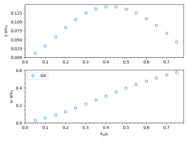
Growth Rates & Frequencies
We can plot the growth rates and real frequencies using the growth_rates.py script in the post_processing directory:
python post_processing/growth_rates.py itg_miller_adiabatic_electrons.out.nc
We can plot the eigenfunctions using the fields.py script in the post_processing directory. The fields diagnostics are stored in the itg_miller_adiabatic_electrons.big.nc file.
python post_processing/fields.py itg_miller_adiabatic_electrons.big.nc